download:original word file
Materials ::
DNA oligonucleotide sequences:
We employ the following DNA oligonucleotides (
![]() ) for experiments (nucleotide ordering is 5’ to 3’):
) for experiments (nucleotide ordering is 5’ to 3’):
Name: Seq. (5’
![]() 3’)
3’)
(b-S1*): 5’ – biotin - GGCGGGAGGATAATCTTAGAACA - 3’
(b-pT(20)-S1*): 5’ – biotin - TTTTTTTTTTTTTTTTTTTT - GGCGGGAGGATAATCTTAGAACA – 3’
(S1*-FAM): 5’ – GGCGGGAGGATAATCTTAGAACA – FAM – 3’
(cvU-S1): 5’ – cvU - TGTTCTAAGATTATCCTCCCGCC - 3’
(b-S2*): 5’ – biotin – GGCGGCTATAACAATTTCATCCA – 3’
(S2*-Cy5): 5’ – GGCGGCTATAACAATTTCATCCA – Cy5 – 3’
(cvU-S2): 5’ – cvU – TGGATGAAATTGTTATAGCCGCC - 3’
(b-S3): 5’ – biotin - GCCCACACTCTTACTTATCGACT - 3’
(b-pT(20)-S3): 5’ – biotin – TTTTTTTTTTTTTTTTTTTT - GCCCACACTCTTACTTATCGACT – 3’
(b-pT(20)-S3*-FAM): 5’ – biotin – TTTTTTTTTTTTTTTTTTTT – AGTCGATAAGTAAGAGTGTGGGC – FAM – 3’
(b-S3-FAM): 5’ – biotin - GCCCACACTCTTACTTATCGACT – FAM - 3’
(S1*-S3*): 5’ - GGCGGGAGGATAATCTTAGAACA – AGTCGATAAGTAAGAGTGTGGGC – 3’
(S2*-S3*): 5’ - GGCGGCTATAACAATTTCATCCA – AGTCGATAAGTAAGAGTGTGGGC – 3’
All oligonucleotides above are derivatives of three “base” sequences {S1, S2, S3} and/or their Watson-Crick complements {S1*, S2*, S3*}. Note that this set
of a base sequences is designed: (1) to have minimal intramolecular secondary structure; and (2) to be “orthogonal” such that intermolecular interactions
between all possible pairs of strands (other than a strand and its Watson-Crick complement, e.g. {S1, S1*}) are minimized. Note that cvU here
refers to a chemically modified nucleobase (5-cyanovinyl-2’-deoxyuridine / CVU) which can be photoligated to an immediately upstream pyrimidine
nucleoside via irradiation at
![]() (i.e. the wavelength corresponding to the highest quantum yield (
(i.e. the wavelength corresponding to the highest quantum yield (
![]() ) for the photocrosslinking reaction).
) for the photocrosslinking reaction).
Methods ::
(Experiment Set 1): Demonstration and quantitation of magnetic bead capture in microplate wells via DNA binding interactions.
(1.1) - Competitive binding assay between b-S3 & b-S3-FAM oligonucleotides for fluorescence readout calibration.
Short summary of experiment:
Here, we incubate streptavidin coated magnetic beads (
![]() diameter ferromagnetic (Fe2O3) iron oxide particles; Magnosphere(TM) MS300/Streptavidin; JSR Lifesciences) with varying ratios of
fluorescent biotinylated b-S3-FAM and non-fluorescent biotinylated b-S3 oligonucleotides. Then, after successive washing steps, we quantitate fluorescence
levels of each bead sample in the wells of a microplate.
diameter ferromagnetic (Fe2O3) iron oxide particles; Magnosphere(TM) MS300/Streptavidin; JSR Lifesciences) with varying ratios of
fluorescent biotinylated b-S3-FAM and non-fluorescent biotinylated b-S3 oligonucleotides. Then, after successive washing steps, we quantitate fluorescence
levels of each bead sample in the wells of a microplate.
This experiment will demonstrate three things: (1) that we can successfully label the aforementioned ferromagnetic beads with oligonucleotides; (2) that we can retain these oligonucleotide labels over the course of several washing steps, where the washing steps are based on magnetic-field capture (which will be demonstrated by fluorescent measurements at the end of the experiment); and (3) that the decided upon concentrations of beads will be sufficient to place fluorescence measurements in the linear range of the detector / scanner we employ (i.e. measurements will fall above the detector noise floor and below the point of detector saturation).
Protocol for experiment [1.1]:
[Step 1] We begin by diluting b-S3 and b-S3-FAM oligonucleotides to a
![]() concentration in
concentration in
![]() SSCT buffer (
SSCT buffer (
![]() mM NaCl,
mM NaCl,
![]() mM sodium citrate, 0.05% Tween-20; pH 7.0).
mM sodium citrate, 0.05% Tween-20; pH 7.0).
[Step 2] We take a
![]() aliquot of the solution containing magnetic beads (
aliquot of the solution containing magnetic beads (
![]() of beads =>
of beads =>
![]() beads in this
beads in this
![]() aliquot) (Magnosphere(TM) MS300/Streptavidin; JSR Lifesciences), set this volume on a magnetic stand for
aliquot) (Magnosphere(TM) MS300/Streptavidin; JSR Lifesciences), set this volume on a magnetic stand for
![]() to collect the magnetic beads at the bottom of the microtube, and finally, we wash off the supernatant. We then additionally wash the magnetic beads (
to collect the magnetic beads at the bottom of the microtube, and finally, we wash off the supernatant. We then additionally wash the magnetic beads (
![]() times) with
times) with
![]() of
of
![]() SSCT buffer, and then resuspend the beads in this same
SSCT buffer, and then resuspend the beads in this same
![]() volume of
volume of
![]() SSCT buffer.
SSCT buffer.
[Step 3] We partition the
![]() buffer into three equivalent
buffer into three equivalent
![]() aliquots (to microtubes assigned the labels 1, 2, & 3). These aliquots are placed on the same magnetic stand as in [step 2], left on the stand for
aliquots (to microtubes assigned the labels 1, 2, & 3). These aliquots are placed on the same magnetic stand as in [step 2], left on the stand for
![]() to allow the magnetic beads in solution to collect on the tube wall at the point nearest to the magnet, and finally, the supernatant in each aliquot is
dumped (taking care not to loss the magnetic bead “pellet”).
to allow the magnetic beads in solution to collect on the tube wall at the point nearest to the magnet, and finally, the supernatant in each aliquot is
dumped (taking care not to loss the magnetic bead “pellet”).
[Step 4] For microtube 1, to a volume of
![]() we add
we add
![]() (=>
(=>
![]() ) of the b-S3-FAM oligonucleotide &
) of the b-S3-FAM oligonucleotide &
![]() (=>
(=>
![]() ) of the b-S3 oligo (achieving a 1:9 ratio of b-S3-FAM to b-S3), for microtube 2, to a volume of
) of the b-S3 oligo (achieving a 1:9 ratio of b-S3-FAM to b-S3), for microtube 2, to a volume of
![]() we add
we add
![]() (=>
(=>
![]() ) of b-S3-FAM &
) of b-S3-FAM &
![]() (=>
(=>
![]() ) of b-S3 (achieving a 3:7 ratio), and finally, for microtube 3, to a volume of
) of b-S3 (achieving a 3:7 ratio), and finally, for microtube 3, to a volume of
![]() we add
we add
![]() (=>
(=>
![]() ) of the b-S3-FAM oligo and no b-S3 (achieving a 1:0 ratio of b-S3-FAM to b-S3).
) of the b-S3-FAM oligo and no b-S3 (achieving a 1:0 ratio of b-S3-FAM to b-S3).
[Step 5] We place the three samples from [step 4] in a microtube rotator for
![]() , then pellet the magnetic beads with a
, then pellet the magnetic beads with a
![]() incubation on the magnetic stand. Once pelleting occurs, the supernatant in each microtube is dumped.
incubation on the magnetic stand. Once pelleting occurs, the supernatant in each microtube is dumped.
[Step 6] To each of microtube we add
![]() of
of
![]() SSCT buffer, and once again, pellet the magnetic beads in each microtube with a
SSCT buffer, and once again, pellet the magnetic beads in each microtube with a
![]() incubation on the magnetic stand, and dump the supernatant in each microtube.
incubation on the magnetic stand, and dump the supernatant in each microtube.
[Step 7] We resuspend the magnetic beads in each microtube with a
![]() volume of
volume of
![]() SSCT buffer.
SSCT buffer.
[Step 8] We partition the
![]() of solution in each microtube {1 through 3} to individual U-shaped wells of a microplate (
of solution in each microtube {1 through 3} to individual U-shaped wells of a microplate (
![]() per well). Note that wells here are “naked” (without a protein coating of e.g. of streptavidin).
per well). Note that wells here are “naked” (without a protein coating of e.g. of streptavidin).
[Step 9] We employ a fluorescent microplate reader FLA-5100 (GE Healthcare Japan) to quantitate the fluorescence level of FAM in each well of the microplate.
Results & analysis for experiment [1.1]:
Figure 1: Fluorescent reads for microplate wells containing
![]() diameter Fe2O3-core magnetic beads incubated with varying concentration ratios of b-S3-FAM and b-S3 oligonucleotides.
diameter Fe2O3-core magnetic beads incubated with varying concentration ratios of b-S3-FAM and b-S3 oligonucleotides.

Fig. 1: Microplate scans from [step 9] of experiment [1.1]. Here, fluorescence levels for each of the
![]()
![]() SSCT buffered solutions of magnetic beads in each well is quantitated using an FLA-5100 fluorescence scanner (GE Healthcare Japan), set to an appropriate
wavelength for the FAM dye labels (
SSCT buffered solutions of magnetic beads in each well is quantitated using an FLA-5100 fluorescence scanner (GE Healthcare Japan), set to an appropriate
wavelength for the FAM dye labels (
![]() ::
::
![]() ). The concentration ratio of b-S3-FAM and b-S3 oligonucleotides (during the biotin-based bead labeling step) is indicated over each well (see RED labels).
We note a clear increase in FAM fluorescence intensity as a function of increasing the b-S3-FAM to b-S3 oligonucleotide concentration ratio during the bead
labeling step.
). The concentration ratio of b-S3-FAM and b-S3 oligonucleotides (during the biotin-based bead labeling step) is indicated over each well (see RED labels).
We note a clear increase in FAM fluorescence intensity as a function of increasing the b-S3-FAM to b-S3 oligonucleotide concentration ratio during the bead
labeling step.
Figure 2: Demonstration of a linear relationship between the molar fraction of b-S3-FAM during bead labeling and arbitrary units of fluorescence.

Fig. 2: The above plot shows quantitated relative values of fluorescence from the microplate scans in Figure 1 normalized to a “blank” well with only
![]() of
of
![]() SSCT buffer and no magnetic beads. The b-S3-FAM to b-S3 ratios for the three data points are again: {1:9, 3:7, 10:0}. Note the observed linear relationship
(i.e. note the regression line
SSCT buffer and no magnetic beads. The b-S3-FAM to b-S3 ratios for the three data points are again: {1:9, 3:7, 10:0}. Note the observed linear relationship
(i.e. note the regression line
![]() b-S3-FAM
b-S3-FAM
![]() with a coefficient of determination
with a coefficient of determination
![]() ), indicating a lack of saturation at upper-end values of the b-S3-FAM ratio (10:0) during the magnetic bead labeling step, as well as the sensitivity to
beads labeled at the lower-end (1:9) ratio of b-S3-FAM.
), indicating a lack of saturation at upper-end values of the b-S3-FAM ratio (10:0) during the magnetic bead labeling step, as well as the sensitivity to
beads labeled at the lower-end (1:9) ratio of b-S3-FAM.
(1.2) – Confirmation of sequence-specific bead docking in microplate wells.
Short summary of experiment:
Here we attempt to demonstrate sequence-specific docking of oligonucleotide coated magnetic beads to specific wells of a microplate labeled with
Watson-Crick complementary oligonucleotides. The basic experiment will consist of labeling streptavidin coated magnetic beads with b-S3 oligonucleotides,
then applying these beads to three different “types” of (here, flat-bottomed & streptavidin coated) microplate wells: (1) wells labeled with b-S3*
oligonucleotides (complementary to the sequences on the b-S3 labeled magnetic beads); (2) wells labeled with b-S1* oligonucleotides (non-complementary to
the strands on the b-S3 labeled magnetic beads); and (3) wells left “blank” (i.e. unlabeled by any oligonucleotide and only filled with
![]() of
of
![]() SSCT buffer).
SSCT buffer).
Protocol for experiment [1.2]:
[Step 1] We begin by preparing separate aliquots of the b-S3, b-S3-FAM, and b-S1* oligonucleotides, where each oligonucleotide is at a
![]() concentration.
concentration.
[Step 2] We pre-wash the wells of the microplate by flushing each well with
![]() of
of
![]() SSCT buffer, and we do this three times.
SSCT buffer, and we do this three times.
[Step 3] We label eight wells of the microplate {“well 1”, “well, 2”, “well 3”, “well 4”, “well 5”, “well 6”, “well 7”, “well 8”}. And in this step, we add the following solutions to these eight wells:
Wells 1 & 5: …we add
![]() of the
of the
![]() solution of the b-S3* strand.
solution of the b-S3* strand.
Wells 2 & 6: …we add
![]() of the
of the
![]() solution of the b-S1* strand.
solution of the b-S1* strand.
Wells 3, 4, 7, & 8: …we add only
![]() of
of
![]() SSCT buffer.
SSCT buffer.
[Step 4] We gently agitate the microplate for
![]() at room temperature (
at room temperature (
![]() -
-
![]() ).
).
[Step 5] In this step, we take a
![]() sample of magnetic beads (
sample of magnetic beads (
![]() pmol of beads) (Magnosphere(TM) MS300/Streptavidin; JSR Lifesciences), set this solution on a magnetic stand for
pmol of beads) (Magnosphere(TM) MS300/Streptavidin; JSR Lifesciences), set this solution on a magnetic stand for
![]() to pellet the beads, and then we dump the supernatant.
to pellet the beads, and then we dump the supernatant.
[Step 6] We wash the beads from the previous step with
![]() of
of
![]() SSCT buffer, and the beads are again pelleted for
SSCT buffer, and the beads are again pelleted for
![]() on a magnetic stand to allow for the removal of the wash solution.
on a magnetic stand to allow for the removal of the wash solution.
[Step 7] We add
![]() of the
of the
![]() b-S3-FAM oligonucleotide solution to the microtube containing the washed magnetic beads, we incubate for
b-S3-FAM oligonucleotide solution to the microtube containing the washed magnetic beads, we incubate for
![]() , and finally we set the solution on a magnetic strand to pellet the beads and dump the supernatant.
, and finally we set the solution on a magnetic strand to pellet the beads and dump the supernatant.
[Step 8] We wash the bead solution from the previous step with
![]() of
of
![]() SSCT buffer, place the microtube with the wash solution on the magnetic stand for
SSCT buffer, place the microtube with the wash solution on the magnetic stand for
![]() to concentrate the beads, and dump the supernatant. We perform this step twice to eliminate the majority of freely diffusing b-S3-FAM oligonucleotide
species.
to concentrate the beads, and dump the supernatant. We perform this step twice to eliminate the majority of freely diffusing b-S3-FAM oligonucleotide
species.
[Step 9] We add
![]() of
of
![]() SSCT buffer to the bead solution from the previous step (where there should be
SSCT buffer to the bead solution from the previous step (where there should be
![]() of pelleted beads, assuming no attrition), and partition this solution into a
of pelleted beads, assuming no attrition), and partition this solution into a
![]() aliquot and a
aliquot and a
![]() aliquot, which we label aliquots 1 & 2, respectively. Note that there will be
aliquot, which we label aliquots 1 & 2, respectively. Note that there will be
![]() of magnetic beads in the
of magnetic beads in the
![]() aliquot (aliquot 1) and
aliquot (aliquot 1) and
![]() of beads in the
of beads in the
![]() aliquot (aliquot 2). We estimate that
aliquot (aliquot 2). We estimate that
![]() of beads should be sufficient to cover the approximately
of beads should be sufficient to cover the approximately
![]() area of a flat-bottomed microplate well, so we should be well in the limit of being able to saturate all potential docking sites in each well with either
aliquot. Finally, for this step, we place both aliquots on the magnetic holder for
area of a flat-bottomed microplate well, so we should be well in the limit of being able to saturate all potential docking sites in each well with either
aliquot. Finally, for this step, we place both aliquots on the magnetic holder for
![]() to pellet the beads, and then we toss the supernatant.
to pellet the beads, and then we toss the supernatant.
[Step 10] To both aliquot 1 & 2 from [step 9], we add
![]() of
of
![]() SSCT buffer.
SSCT buffer.
[Step 11] At this point, we wait until the
![]() agitation period for the microplate (see [step 3]) comes to an end, and then we wash all wells of the microplate three times, each time adding and removing
a fresh
agitation period for the microplate (see [step 3]) comes to an end, and then we wash all wells of the microplate three times, each time adding and removing
a fresh
![]() volume of
volume of
![]() SSCT buffer (using a pipette).
SSCT buffer (using a pipette).
[Step 12] Taking now the two aliquots from [Step 9] (aliquot 1 consisting of a
![]() solution containing
solution containing
![]() of beads; aliquot 2 consisting of a
of beads; aliquot 2 consisting of a
![]() solution containing
solution containing
![]() of beads), we add individual
of beads), we add individual
![]() volumes of aliquot 1 to wells {1, 2, 3} of the microplate, and individual
volumes of aliquot 1 to wells {1, 2, 3} of the microplate, and individual
![]() volumes of aliquot 2 to each of wells {5, 6, 7} of the microplate. To the “blank” wells 4 & 8, we simply add
volumes of aliquot 2 to each of wells {5, 6, 7} of the microplate. To the “blank” wells 4 & 8, we simply add
![]() of
of
![]() SSCT buffer. Here, the assumed amount of beads added to wells {1, 2, 3} is
SSCT buffer. Here, the assumed amount of beads added to wells {1, 2, 3} is
![]() , and the assumed amount of beads added to wells {5, 6, 7} is
, and the assumed amount of beads added to wells {5, 6, 7} is
![]() .
.
[Step 13] We place the microplate from the preceding steps on a rotator (operating at
![]() ), and under these conditions we incubate at room temperature for
), and under these conditions we incubate at room temperature for
![]() . Once this incubation period is over, we pipette off the supernatant in each well.
. Once this incubation period is over, we pipette off the supernatant in each well.
[Step 14] We perform two sequential types of wash processes. For the first wash process, we add
![]() of
of
![]() SSCT buffer to each well of the microplate, then pipette off the wash solution. This first wash process is repeated three times. For the second wash
process, we do much the same thing, adding
SSCT buffer to each well of the microplate, then pipette off the wash solution. This first wash process is repeated three times. For the second wash
process, we do much the same thing, adding
![]() to each well of the microplate, however here, we pipette this solution up-and-down five times before finally pipetting off and disposing of the wash
buffer.
to each well of the microplate, however here, we pipette this solution up-and-down five times before finally pipetting off and disposing of the wash
buffer.
[Step 15] We add
![]() of
of
![]() SSCT buffer to each well of the microplate.
SSCT buffer to each well of the microplate.
[Step 16] We take fluorescence scans of the microplate, setting the FLA-5100 scanner (in this case) to take into account the proper excitation and emission
spectra for the FAM dye on the 3’ termini of b-S3-FAM oligonucleotides (
![]() ::
::
![]() ).
).
Results & analysis for experiment [1.2]:
Schematic 1: Representation of microplate well specifications.
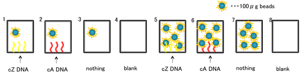
Schematic 1:
As illustrated in the above diagram, wells 1 and 5 contain b-S3* oligonucleotides, and wells 2 and 6 contain b-S1* oligonucleotides. Here, the assumed
amount of beads added to wells {1, 2, 3} is
![]() , and the assumed amount of beads added to wells {5, 6, 7} is
, and the assumed amount of beads added to wells {5, 6, 7} is
![]() .
.
Figure 3: Fluorescent reads for microplate wells with contents indicated in [Schematic 1].
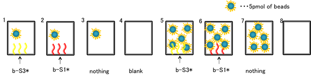
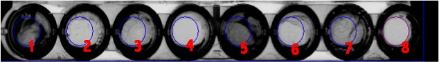
Fig. 3: Microplate scans from [step 16] of experiment [1.2]. Here, in he context of a
![]() volume of
volume of
![]() SSCT buffer, the FAM fluorescence level in each well is quantitated using an FLA-5100 fluorescence scanner (GE Healthcare Japan), set to an appropriate
wavelength for the FAM dye labels (
SSCT buffer, the FAM fluorescence level in each well is quantitated using an FLA-5100 fluorescence scanner (GE Healthcare Japan), set to an appropriate
wavelength for the FAM dye labels (
![]() ::
::
![]() ). Note that wells 1 & 5, labeled with b-S3* oligos (i.e. Watson-Crick complements to the b-S3-FAM oligos on all beads) exhibit qualitatively HIGH
levels of fluorescence in comparison to all other wells. Moreover, fluorescence levels in wells 1 & 5 appear comparable (qualitatively speaking), this
being the case despite the five-fold greater number of beads added to well 5. Note that wells 3 & 7 show slightly elevated levels of fluorescence
relative to wells 2 & 6 (which are wells labeled with b-S1* oligos, orthogonal / non-complementary to the b-S3-FAM oligos on all beads). Finally, note
that apparent lack of fluorescence in the “blank” wells, where no beads or other dye-labeled oligonucleotides are added (indicating little to no
fluorescent background due to the microplate or the
). Note that wells 1 & 5, labeled with b-S3* oligos (i.e. Watson-Crick complements to the b-S3-FAM oligos on all beads) exhibit qualitatively HIGH
levels of fluorescence in comparison to all other wells. Moreover, fluorescence levels in wells 1 & 5 appear comparable (qualitatively speaking), this
being the case despite the five-fold greater number of beads added to well 5. Note that wells 3 & 7 show slightly elevated levels of fluorescence
relative to wells 2 & 6 (which are wells labeled with b-S1* oligos, orthogonal / non-complementary to the b-S3-FAM oligos on all beads). Finally, note
that apparent lack of fluorescence in the “blank” wells, where no beads or other dye-labeled oligonucleotides are added (indicating little to no
fluorescent background due to the microplate or the
![]() SSCT buffer).
SSCT buffer).
Figure 4: Quantitative FAM fluorescence emission in wells {1, 2, 3, 5, 6, 7} from [Schematic 1].
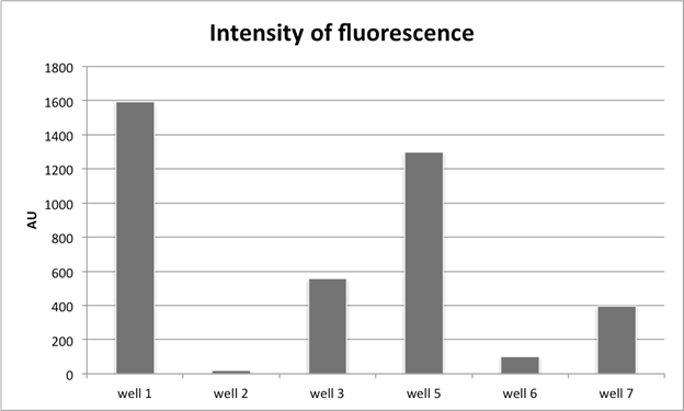
Fig. 4:
Here we show quantitative fluorescent reads for wells {1, 2, 3, 5, 6, 7}, all of which are normalized to the A.U. value of well 8. Note here three
important points: (1) that the relative fluorescence ratios between wells {1, 2, 3} appear to correspond well to the relative fluorescence ratios exhibited
by wells {5, 6, 7} (i.e. the same qualitative behavior is exhibited for both sets of wells); (2) higher A.U. counts for Watson-Crick specific bead capture
appear to occur in well 1 relative to well 5 (where one adds
![]() vs.
vs.
![]() of beads); and (3) that wells 3 & 7, where no oligos decorate the surface of the well, show increased fluorescence (presumably corresponding to
non-specific bead capture) relative to wells 2 & 6 where non-complementary b-S1* oligos coat the bottom of the well. This is a very interesting
phenomena to us, which may be due to electrostatic or other “polymer brush” based effects leading to the non-complementary oligos blocking non-specific
binding of beads to the bottom of the microplate well (i.e. in wells 2 & 6). However, further study is of course required to say anything conclusive on
this matter (e.g. it’s unclear why well 3 would have higher fluorescence count than well 7 where 5-fold fewer beads were added).
of beads); and (3) that wells 3 & 7, where no oligos decorate the surface of the well, show increased fluorescence (presumably corresponding to
non-specific bead capture) relative to wells 2 & 6 where non-complementary b-S1* oligos coat the bottom of the well. This is a very interesting
phenomena to us, which may be due to electrostatic or other “polymer brush” based effects leading to the non-complementary oligos blocking non-specific
binding of beads to the bottom of the microplate well (i.e. in wells 2 & 6). However, further study is of course required to say anything conclusive on
this matter (e.g. it’s unclear why well 3 would have higher fluorescence count than well 7 where 5-fold fewer beads were added).
(1.3) – Investigating the impact of linker (spacer) addition to the bead and well-surface functionalizing oligonucleotides from experiment [2.1].
Short summary of experiment: Here we repeat the basic experiment from [1.2] (though without the non-complementary oligo controls), swapping the b-S3*-FAM oligo for an otherwise identical oligo b-pT(20)-S3*-FAM strand with a 20-nt polythymidine linker immediately downstream of the biotin label and immediately upstream of the basic S3* sequence. Likewise, we swap the well plate functionalizing oligo b-S3 with “b-pT(20)-S3, which similarly has a 20nt polythymidine linker between the biotin label and the basic S3 sequence (which is again Watson-Crick complementary to the S3* basic sequences tethered from the beads).
Schematic 2: Beads attaching to Watson-Crick complements in microplate wells, where microplate well “anchor sequences” are tethered from a surface-conjugated (single-stranded) 20nt polythymidine spacers.
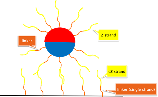
Schematic 2:
This is the basic system we wish to test. Here, b-pT(20)-S3*-FAM oligos modifying the
![]() diameter ferromagnetic beads act to anchor the bead (in a sequence specific manner as per the results of [2.1]) to b-pT(20)-S3 oligos
modifying the surface of a flat-bottomed well.
diameter ferromagnetic beads act to anchor the bead (in a sequence specific manner as per the results of [2.1]) to b-pT(20)-S3 oligos
modifying the surface of a flat-bottomed well.
Schematic 3: Beads attaching to Watson-Crick complements in microplate wells, where microplate well “anchor sequences” are tethered from a surface-conjugated 20nt dsDNA duplexes.
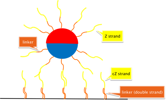
Schematic 3: This is the minor variant of [Schematic 2] wherein a 20nt polyadenine linker is hybridized to ONLY b-pT(20)-S3 “docking” strands on the surface at the bottom of a microplate well. Critically here, we hybridize the 20nt polyadenine complement to the aforementioned polythymidine linkers PRIOR to biotin conjugation to streptavidin molecules on the well surface.
Protocol for experiment [1.3]:
The protocol here is almost that same as that for [1.2], with the following important differences:
(1) We skip the necessary steps where non-complementary b-S1 strands are employed to set up controls for sequence specific bead docking.
(2) We change the density of oligonucleotides during the bead functionalization step from
![]() (employed in experiment [1.2]) to
(employed in experiment [1.2]) to
![]() .
.
(3) For the experiment shown in [Schematic 3], complements to the polythymidine linkers on the microplate well surface are pre-annealed to
20nt polyadenine spacer complements PRIOR to well surface functionalization. More specifically, b-pT(20)-S3 oligos and 20nt polyadenine complements are
mixed at a 1:1 ration, where each oligo is at a
![]() concentration, and annealed using a thermocycler that runs a cooling routine initiating from
concentration, and annealed using a thermocycler that runs a cooling routine initiating from
![]() .
.
Results & analysis for experiment [1.3]:
Figure 5: Fluorescence scans for kinetic study of b-pT(20)-S3*-FAM oligo functionalized bead docking to wells decorated with b-pT(20)-S3 Watson-Crick complementary oligos.
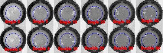
Fig. 5:
Here we modify [step 13] from the protocol for experiment [1.2] to take timepoints at {0, 5, 10, 20, 30, 60} minutes. For each timepoint,
we allow
![]() of beads the indicated amount of time in minutes to attach to their Watson-Crick complements functionalizing the well surfaces. A timepoint is ended or
terminated when one executes the wash steps beginning at the end of [step 13] (again, in the protocol for [1.2]). This experiment is used
to estimate (presumably sequence specific) bead docking kinetics.
of beads the indicated amount of time in minutes to attach to their Watson-Crick complements functionalizing the well surfaces. A timepoint is ended or
terminated when one executes the wash steps beginning at the end of [step 13] (again, in the protocol for [1.2]). This experiment is used
to estimate (presumably sequence specific) bead docking kinetics.
Figure 6: Fluorescence intensity vs. binding time for ssDNA functionalized beads docking to wells decorated with Watson-Crick complementary oligos.
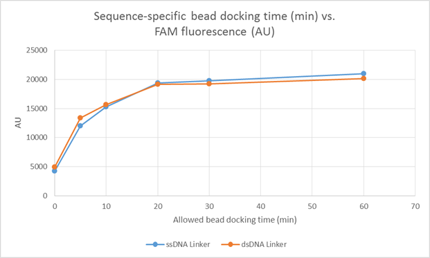
Fig. 6:
Here we show quantitative and normalized values for FAM fluorescence as a function of the amount of time
![]() of beads is afforded to dock to Watson-Crick complementary oligonucleotides decorating the surface of microplate wells. As discussed in the context of [Figure 5], this experiment represents an extension of [step 13] from experiment [1.2], where, at the end of a given
timepoint, a pipette is used to remove the buffer (and thus, freely diffusing beads) from the microplate. Notice here that we compare two sets of
experiments: (1) experiments done with 20nt polythymidine sequences tethering bead-complementary sequences to the floor of the microplate wells ( BLUE); (2) experiments done with 20nt dsDNA (polythymidine :: polyadenine) sequences tethering the same bead-complementary sequences as in
(1) to the floor of the microplate wells (RED). Notice also that the single- and double-stranded tethers allow for approximately the same
bead binding kinetics.
of beads is afforded to dock to Watson-Crick complementary oligonucleotides decorating the surface of microplate wells. As discussed in the context of [Figure 5], this experiment represents an extension of [step 13] from experiment [1.2], where, at the end of a given
timepoint, a pipette is used to remove the buffer (and thus, freely diffusing beads) from the microplate. Notice here that we compare two sets of
experiments: (1) experiments done with 20nt polythymidine sequences tethering bead-complementary sequences to the floor of the microplate wells ( BLUE); (2) experiments done with 20nt dsDNA (polythymidine :: polyadenine) sequences tethering the same bead-complementary sequences as in
(1) to the floor of the microplate wells (RED). Notice also that the single- and double-stranded tethers allow for approximately the same
bead binding kinetics.
(2.1) – Pilot for the creation of bichromatic ferromagnetic beads.
Short summary of experiment: This experiment constitutes our proof-of-principle that photoligation with 5-cyanovinyl-2’-deoxyuridine can work on the surface of beads to direct covalent attachment of oligonucleotides (as evidenced by the ability of the ligated complexes to remain intact during the course of an alkaline denaturation step). In particular, here we label our beads with the b-S3 oligo via the protocol outlined in section [1.1], hybridize the (S1*-S3*) oligo to the b-S3 bead conjugated oligos, and then perform photoligation between CVU-S1 and the b-S3 strand. Once this is done, b-S3 and CV U-S1 will form a covalent product held to the bead by a biotin-streptavidin bond.
Protocol for experiment [2.1]:
[Step 1] We begin by forming separate
![]() aliquots of the b-S3, CVU-S1, S1*-S3*, & S1*-FAM oligos in
aliquots of the b-S3, CVU-S1, S1*-S3*, & S1*-FAM oligos in
![]() SSCT buffer. The prefix “CVU” is again meant to refer to the chemical group 5-cyanovinyl-2’-deoxyuridine.
SSCT buffer. The prefix “CVU” is again meant to refer to the chemical group 5-cyanovinyl-2’-deoxyuridine.
[Step 2] We add
![]() (
(
![]() ) of magnetic bead solution to a microtube. We set it on a magnetic stand for
) of magnetic bead solution to a microtube. We set it on a magnetic stand for
![]() to pellet the magnetic beads, and then we dump the supernatant.
to pellet the magnetic beads, and then we dump the supernatant.
[Step 3] We perform a single washing step for the bead sample from the previous step by adding
![]() of
of
![]() SSCT buffer to the tube, setting the tube on the magnetic stand for
SSCT buffer to the tube, setting the tube on the magnetic stand for
![]() to pellet the beads, and then dumping the supernatant fluid.
to pellet the beads, and then dumping the supernatant fluid.
[Step 4] We add
![]() of the b-S3 aliquot (from [step 1]) to the bead solution. We call this mixture: {beads, b-S3}.
of the b-S3 aliquot (from [step 1]) to the bead solution. We call this mixture: {beads, b-S3}.
[Step 5] We incubate the sample from the previous step ({beads, b-S3}) at room temperature for
![]() , then place the tube on the magnetic stand to pellet the beads, and once this is done, we dump the supernatant.
, then place the tube on the magnetic stand to pellet the beads, and once this is done, we dump the supernatant.
[Step 6] We wash the beads from the sample in the previous step twice (i.e. we wash {beads, b-S3} twice), each time adding
![]() of
of
![]() SSCT buffer, then placing the tube on a magnetic stand for
SSCT buffer, then placing the tube on a magnetic stand for
![]() to pellet the beads and to allow for the dumping of the supernatant.
to pellet the beads and to allow for the dumping of the supernatant.
[Step 7] After the two washes from the previous step, we add another
![]() volume of (here)
volume of (here)
![]() SSCT buffer to the tube containing the sample {beads, b-S3}. Set aside
SSCT buffer to the tube containing the sample {beads, b-S3}. Set aside
![]() in a tube labeled “for positive control”.
in a tube labeled “for positive control”.
[Step 8] We mix together
![]() of the S1*-S3* strand at
of the S1*-S3* strand at
![]() and
and
![]() of the CVU-S1 strand at
of the CVU-S1 strand at
![]() , and anneal the two strands together via the use of a thermocycler (ramping down from
, and anneal the two strands together via the use of a thermocycler (ramping down from
![]() to room temperature). We call the tube containing this annealed product: {CVU-S1, S1*-S3*}.
to room temperature). We call the tube containing this annealed product: {CVU-S1, S1*-S3*}.
[Step 9] We mix together
![]() of the {CVU-S1, S1*-S3*} tube (where strands are now at
of the {CVU-S1, S1*-S3*} tube (where strands are now at
![]() ) and tube containing the {beads, b-S3} from [step 7], and incubate this new mixture {beads, b-S3, CVU-S1, S1*-S3*} at room temperature for
) and tube containing the {beads, b-S3} from [step 7], and incubate this new mixture {beads, b-S3, CVU-S1, S1*-S3*} at room temperature for
![]() .
.
[Step 10] Here, we take five
![]() aliquots from the {beads, b-S3, CVU-S1, S1*-S3*} mixture generated during the previous step, and label these aliquots {0, 30, 60, 90, 120}.
Next, we irradiate each aliquot with
aliquots from the {beads, b-S3, CVU-S1, S1*-S3*} mixture generated during the previous step, and label these aliquots {0, 30, 60, 90, 120}.
Next, we irradiate each aliquot with
![]() light for a time period in minutes corresponding to the tube’s label (e.g. the tube with label “60” would be subject to continuous irradiation over the
course of an hour).
light for a time period in minutes corresponding to the tube’s label (e.g. the tube with label “60” would be subject to continuous irradiation over the
course of an hour).
[Step 11] We wash each aliquot three times, each time applying
![]() of
of
![]() SSCT, setting the test tubes on the magnetic rack to pellet the beads in each tube, and then pouring off the supernatant in each tube.
SSCT, setting the test tubes on the magnetic rack to pellet the beads in each tube, and then pouring off the supernatant in each tube.
[Step 12] We resuspend each tube in
![]() NaOH (
NaOH (
![]() ) for precisely
) for precisely
![]() . To allow for immediate discard of the supernatant after the
. To allow for immediate discard of the supernatant after the
![]() alkaline shock, we keep all aliquots on the magnetic stand. As an alkaline shock of this severe nature should be sufficient to melt any 20nt or so DNA
duplex, it provides us a test for whether or not the CVU-S1 oligo is effectively photoligated to the adjacent b-S3 strand as directed by the
native version of the {beads, b-S3, CVU-S1, S1*-S3*} complex. Note that regardless of what occurs with respect to the photoligation, during the
alkaline shock S1*-S3* should dissociate, float away, and become lost forever.
alkaline shock, we keep all aliquots on the magnetic stand. As an alkaline shock of this severe nature should be sufficient to melt any 20nt or so DNA
duplex, it provides us a test for whether or not the CVU-S1 oligo is effectively photoligated to the adjacent b-S3 strand as directed by the
native version of the {beads, b-S3, CVU-S1, S1*-S3*} complex. Note that regardless of what occurs with respect to the photoligation, during the
alkaline shock S1*-S3* should dissociate, float away, and become lost forever.
[Step 13] We now perform a wash where we do the following procedure three times: we add
![]() of
of
![]() SSCT buffer to each aliquot (after dumping of the alkaline solution), we then place the aliquot tubes on the magnetic stand for
SSCT buffer to each aliquot (after dumping of the alkaline solution), we then place the aliquot tubes on the magnetic stand for
![]() to pellet the beads, and we then discard the supernatant.
to pellet the beads, and we then discard the supernatant.
[Step 14] To every aliquot we add
![]() of the S1*-FAM oligonucleotide and incubate at room temperature for
of the S1*-FAM oligonucleotide and incubate at room temperature for
![]()
[Step 15] We repeat exactly [step 13].
[Step 16] We create a positive control by mixing
![]() of S1*-FAM at
of S1*-FAM at
![]() with
with
![]() of the “for positive bead control” solution from [step 7]. Everything should be in
of the “for positive bead control” solution from [step 7]. Everything should be in
![]() SSCT buffer for this step.
SSCT buffer for this step.
[Step 17] We add
![]() to (now) all six aliquots (the new sixth one being the positive control).
to (now) all six aliquots (the new sixth one being the positive control).
[Step 18] We add each aliquot to individual wells of a microplate (adding only
![]() per well).
per well).
[Step 19] We scan the microplate from [step 18] using a fluorescence detector for microplates.
Results & analysis for experiment [2.1]:
Figure 7: Fluorescence scans for CVU photoligation time point samples.

Fig. 7:
If a CVU photoligation event is successful, it should uniquely be possible to capture S1*-FAM, and retain this oligo during the multiple washes
specified in the experimental protocol. Here we see what appears to be fairly strong evidence of a direct correlation between
![]() irradiation times and photoproduct yields.
irradiation times and photoproduct yields.
Figure 8: CVU photoligation product yield on beads vs. time.
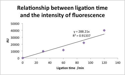
Fig. 8:
Here, extending the discussion from [Figure 7] we see a clear linear relationship (with a coefficient of determination
![]() ) between irradiation time and CVU crosslinking yields. This relationship may of course not extend considerably beyond
) between irradiation time and CVU crosslinking yields. This relationship may of course not extend considerably beyond
![]() of irradiation time.
of irradiation time.
(2.2) – Determination of absolute concentrations from FLA-5100 (GE Healthcare Japan) plate reader fluorescence measurements.
Short summary of experiment: In all previous experiments {[1.1], [1.2], [1.3], & [2.1]} we’ve spoken of FLA-5100 (GE Healthcare Japan) microplate scanner fluorescence measurements in terms of “Arbitrary Units” (or “AU”). Here we perform measurements to precisely determine the relationship between the concentration of FAM- or Cy5- labeled oligonucleotides, and these fluorescence “AU” units (for this particular scanner & with these particular plates). All this will require will be setting up wells on the microplate with various concentrations of FAM and Cy5, recording relative fluorescence measurements, and doing some straightforward linear regression analysis.
Protocol for experiment [2.2]:
[Step 1] We begin by setting up individual and separate
![]() volumes of
volumes of
![]() SSCT buffered FAM and Cy5 labeled oligonucleotides, at concentrations of: {
SSCT buffered FAM and Cy5 labeled oligonucleotides, at concentrations of: {
![]() nM,
nM,
![]() nM,
nM,
![]() pM,
pM,
![]() pM}.
pM}.
[Step 2] We add
![]() of
of
![]() SSCT buffer to each well of the microplate, and pipette off the volume. We repeat this step a total of three times.
SSCT buffer to each well of the microplate, and pipette off the volume. We repeat this step a total of three times.
[Step 3] To individual microplate wells, we add
![]() of each of the solutions prepared in [Step 1].
of each of the solutions prepared in [Step 1].
[Step 4] We scan the plate with the FLA-5100 scanner.
Results & analysis for experiment [2.2]:
Figure 9: Direct FLA-5100 scans of microplate wells with varying concentrations of FAM (top set) & Cy5 (bottom set).
FAM SCANS (BELOW):
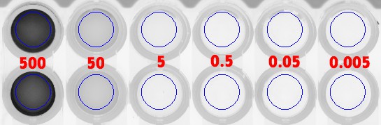
CY5 SCANS (BELOW):
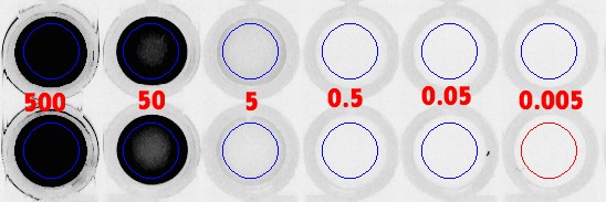
Fig. 9:
These are original microplate well scans from the FLA-5100 fluorescence scanner (GE Healthcare Japan). Note that there are four rows of wells here, the top
two of which are scans for FAM-labeled oligos (here, S1*-FAM), and the bottom two of which are scans for Cy5-labeled oligos (here, S2*-Cy5). Now, moving
from left to right, the overlaid (RED) values represent the concentration (in units: nanomolar) for the dye label in each well: {
![]() nM,
nM,
![]() nM,
nM,
![]() pM,
pM,
![]() pM}. Wells at position
pM}. Wells at position
![]() in the first two rows, or in the last two rows, are identical samples of one-another, which are averaged for the collection of a data point at a particular
FAM or Cy5 label concentration.
in the first two rows, or in the last two rows, are identical samples of one-another, which are averaged for the collection of a data point at a particular
FAM or Cy5 label concentration.
Figure 10: The relationship between FLA-5100 recorded FAM fluorescence in the well of a plate and its actual molar concentration.
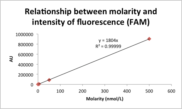
Fig. 10: Here we use data collected from plate measurements (see [Figure 9]) to extrapolate, via simple linear regression, the relationship between the FLA-5100’s units of AU for the FAM dye and the dye’s actual molar concentration. Specifically, and noting the impressive coefficient of correlation we achieve, we suggest the following relationship:
![]()
Figure 11: The relationship between FLA-5100 recorded Cy5 fluorescence in the well of a plate and its actual molar concentration.
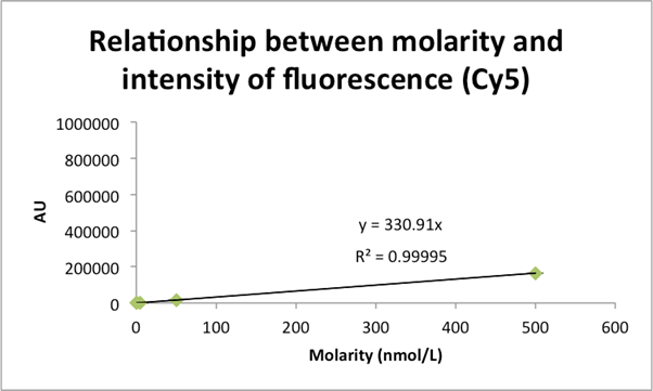
Fig. 11: Just as in [Figure 10], we use data collected from plate measurements (see [Figure 9]) to extrapolate, via simple linear regression, the relationship between the FLA-5100’s units of AU for the Cy5 dye and the dye’s actual molar concentration. Specifically, and noting the impressive coefficient of correlation we achieve, we suggest the following relationship:
![]()
Also notice the very different definitions for AU depending on the choice of dye and/or the dye emission/excitation spectrum --- e.g. here one unit of AU
for TAM is worth
![]() units of AU for Cy5. The lesson here is that one must always calibrate their scanner or generate a reference for any novel dye choice.
units of AU for Cy5. The lesson here is that one must always calibrate their scanner or generate a reference for any novel dye choice.
(2.3) – A first light: proof of the asymmetric bead functionalization protocol.
Short summary of experiment:
Here we initiate the first pilot experiment for the creation of ferromagnetic (Fe2O3) beads with “bichromatic” features. In
particular, here we are able to show that
![]() irradiation --- at power densities and for durations necessary to allow for 5-cyanovinyl-2’-deoxyuridine (CVU) photocrosslinking to a nucleic
acid pyrimidine base --- can be effectively blocked by the thickness (
irradiation --- at power densities and for durations necessary to allow for 5-cyanovinyl-2’-deoxyuridine (CVU) photocrosslinking to a nucleic
acid pyrimidine base --- can be effectively blocked by the thickness (
![]() ) and opacity of the beads we have thus far been working with, allowing us to asymmetrically functionalize their hemispheres (and by this action making
them “bichromatic”).
) and opacity of the beads we have thus far been working with, allowing us to asymmetrically functionalize their hemispheres (and by this action making
them “bichromatic”).
In a bit more detail, we first use biotin-streptavidin interactions to decorate the flat-bottomed surfaces of microplate wells with the b-pT(20)-S3* oligo (consisting of the basic S3 sequence on a 20nt polythymidine tether), we likewise prepare b-pT(20)-S3 labeled beads (as per experiment [1.1], if one swaps b-pT(20)-S3 for b-S3-FAM), and then sequence specifically dock these beads to the bottom of a subset of the wells in the microplate (in the same spirit as experiment [1.2]). Once we’ve sequence specifically dock the beads to the bottom of the microplate wells, we can then hybridize on a pre-annealed {S1*-S3* :: CVU-S1} complex.
And this is where the magic comes in. Micron-sized metallic colloids are, in most cases, quite a bit better than nanoscale objects at scattering and
absorbing light (the latter property due to the finely spaced energy levels in the conduction band for most metals). Thus, if we irradiate the beads with a
top-down source of directional (not coherent)
![]() near-UV light, we’ll form a covalent linkage between CVU-S1 and the 3’ termini of the b-pT(20)-S3 sequence on the beads --- but ONLY on the
bead’s more exposed hemisphere pointing away from the surface!
near-UV light, we’ll form a covalent linkage between CVU-S1 and the 3’ termini of the b-pT(20)-S3 sequence on the beads --- but ONLY on the
bead’s more exposed hemisphere pointing away from the surface!
Now, once the beads have a specific sequence on their one hemisphere, microplate wells (in just the same manner as before) can be prepared to dock these
beads only on that one side. Thus, the formally shielded side will now flip up towards the
![]() source. At this point, we decided to form a pre-annealed {S2*-S3* :: CVU-S2} complex, and demonstrate (ultimately using S2*-Cy5 as a probe) that
the opposite hemisphere to the one formally functionalized could be specifically decorated with a new oligonucleotide (i.e. CVU-S2).
source. At this point, we decided to form a pre-annealed {S2*-S3* :: CVU-S2} complex, and demonstrate (ultimately using S2*-Cy5 as a probe) that
the opposite hemisphere to the one formally functionalized could be specifically decorated with a new oligonucleotide (i.e. CVU-S2).
Protocol for experiment [2.3]:
[Step 1] We form
![]() stocks (in
stocks (in
![]() SSCT buffer) of the following oligonucleotides: {b-pt(20)-S3, ,b-pt(20)-S3*, S3*-S1*, S3*-S2*, cvU-S1, cvU-S2, S1*-FAM, S2*-Cy5, b-pt(20)-S1*, b-S1*,
b-S2*, b-S3-FAM}.
SSCT buffer) of the following oligonucleotides: {b-pt(20)-S3, ,b-pt(20)-S3*, S3*-S1*, S3*-S2*, cvU-S1, cvU-S2, S1*-FAM, S2*-Cy5, b-pt(20)-S1*, b-S1*,
b-S2*, b-S3-FAM}.
[Step 2] We label a set of four microtubes with the labels: {3-44, 3-16, 18-29, 31-44}.
[Step 3] We prewash the individual wells of a flat-bottomed (streptavidinated) microplate with
![]() of
of
![]() SSCT buffer (pipetting off the individual volumes after their application).
SSCT buffer (pipetting off the individual volumes after their application).
[Step 4] To each well on the microplate, we add
![]() of the b-pT(20)-S3* oligo stock at
of the b-pT(20)-S3* oligo stock at
![]() (i.e. we add
(i.e. we add
![]() of this oligo to each well of the microplate).
of this oligo to each well of the microplate).
[Step 5] We allow the plate to incubate at room temperature (
![]() ) for
) for
![]() , spinning the plate at
, spinning the plate at
![]() during this time.
during this time.
[Step 6] Once the incubation from the previous step is finished, we wash each well by adding
![]() of
of
![]() SSCT buffer, pipette off the wash solution. We repeat this process three times.
SSCT buffer, pipette off the wash solution. We repeat this process three times.
[Step 7] We take a
![]() solution of magnetic beads (Magnosphere(TM) MS300/Streptavidin; JSR Lifesciences) (
solution of magnetic beads (Magnosphere(TM) MS300/Streptavidin; JSR Lifesciences) (
![]() of beads), pellet the beads by placing this volume on our magnetic stand for
of beads), pellet the beads by placing this volume on our magnetic stand for
![]() , then toss the supernatant.
, then toss the supernatant.
[Step 8] We add a volume of
![]() of
of
![]() SSCT buffer to the pelleted beads from the previous step, pipette this volume up and down
SSCT buffer to the pelleted beads from the previous step, pipette this volume up and down
![]() times, pellet the beads again by setting the volume on a magnetic stand for
times, pellet the beads again by setting the volume on a magnetic stand for
![]() , then we toss the supernatant. We repeat this process a total of three times.
, then we toss the supernatant. We repeat this process a total of three times.
[Step 9] We add
![]() of the b-pt(20)-S3 solution, at
of the b-pt(20)-S3 solution, at
![]() concentration, to the pelleted beads from the previous step, and incubate the mix for
concentration, to the pelleted beads from the previous step, and incubate the mix for
![]() at room temperature.
at room temperature.
[Step 10] We set the microtube from the previous step on our magnetic stand for
![]() , pelleting the beads and allowing us to toss the supernatant.
, pelleting the beads and allowing us to toss the supernatant.
[Step 11] We add a volume of
![]() of
of
![]() SSCT buffer (NOT
SSCT buffer (NOT
![]() SSCT buffer as in [step 8]) to the pelleted beads from the previous step, pipette this volume up and down
SSCT buffer as in [step 8]) to the pelleted beads from the previous step, pipette this volume up and down
![]() times, pellet the beads again by setting the volume on a magnetic stand for
times, pellet the beads again by setting the volume on a magnetic stand for
![]() , then we toss the supernatant. We repeat this process a total of three times.
, then we toss the supernatant. We repeat this process a total of three times.
[Step 12] We
![]() of
of
![]() SSCT buffer to the pelleted beads from the previous step, and transfer
SSCT buffer to the pelleted beads from the previous step, and transfer
![]() of this volume to each of two wells on the microplate.
of this volume to each of two wells on the microplate.
[Step 13] Rotate the plate at
![]() for
for
![]() at room temperature (
at room temperature (
![]() ).
).
[Step 14] Wash each (used) well of the plate three times with
![]() per well of
per well of
![]() SSCT buffer (pipetting each volume off after its application).
SSCT buffer (pipetting each volume off after its application).
[Step 15] We mix together
![]() of S1*-S3* at
of S1*-S3* at
![]() and
and
![]() of CVU-S1 at
of CVU-S1 at
![]() . A thermal anneal is then conducted using a thermocycler, where a ramp initiated at
. A thermal anneal is then conducted using a thermocycler, where a ramp initiated at
![]() returns to room temperature over the course of
returns to room temperature over the course of
![]() .
.
[Step 16] We add
![]() of the annealed solution from the previous step to
of the annealed solution from the previous step to
![]() of
of
![]() SSCT buffer, and partition
SSCT buffer, and partition
![]() volumes of this solution to the two “in use” wells on the microplate (which should have been the washed wells from [step 14]).
volumes of this solution to the two “in use” wells on the microplate (which should have been the washed wells from [step 14]).
[Step 17] We shake & rotate the plate at
![]() for
for
![]() at room temperature (
at room temperature (
![]() ), allowing the S1*-S3* and b-pt(20)-S3 strands to hybridize.
), allowing the S1*-S3* and b-pt(20)-S3 strands to hybridize.
[Step 18] We irradiate the wells on the microplate with
![]() light for
light for
![]() minutes at room temperature (
minutes at room temperature (
![]() ). This should lead to photocrosslinking (via [2+2] photocycloaddition) of the CVU-S1 oligo to the 3’-most base of the b-pt(20)-S3 oligo (which
must be a pyrimidine, and is in this case deoxythymidine).
). This should lead to photocrosslinking (via [2+2] photocycloaddition) of the CVU-S1 oligo to the 3’-most base of the b-pt(20)-S3 oligo (which
must be a pyrimidine, and is in this case deoxythymidine).
[Step 19] We pipette off the volume of the irradiated wells from [step 18], and perform an alkaline “shock” by adding a
![]() NaOH buffer with
NaOH buffer with
![]() NaOH. This alkaline shock will denature all DNA, and will presumably begin to denature the streptavidin coupling the biotin-labeled oligos to the bead
surface --- so it’s important to only have the beads exposed to alkaline conditions for
NaOH. This alkaline shock will denature all DNA, and will presumably begin to denature the streptavidin coupling the biotin-labeled oligos to the bead
surface --- so it’s important to only have the beads exposed to alkaline conditions for
![]() . Once this minute has passed, pipette the solution out of the well and transfer the beads to a microtube.
. Once this minute has passed, pipette the solution out of the well and transfer the beads to a microtube.
Now:
① Remove S1*-S1 and S3*-S3 binding by alkaline denaturation.
② Transfer the beads to a microtube.
③ Wash beads in the way of ⑦. The amount of 2 x SSCT buffer is 100 μL. Now,S1 strand would be immobilized on the hemisphere of beads.
④ Set microtubes to a magnet for 1 minute, and dump supernatant fluid.
⑤ Subject alkaline denaturation.
⑥ Wash beads in the way of ⑳. Here, the amount of 2 x SSCT buffer is 100 μL.
⑦ Immobilize b-S1* strand to a well of the streptavidin plate in the way of ③-⑥.
⑧ Transefer the beads to the well with b-S1* strand.
⑨ Shake the plate for 1 hour by 70 rpm at room temperature. A and cA strand hybridize.
⑩ Anneal 10 μL of S2*-S3* and 10 μL of cvU-S2 strand for 10 minutes.
⑪ Add 10 μl/well of 27 to the wells with beads.
⑫ Shake the plate for 10 minute by 70 rpm at room temperature.
⑬ Shed 366 nm of UV light for 20 minutes to the well at room temperature.
⑭ Remove S1*-S1 and S2*-S2 binding by alkaline denaturation.
⑮ Transfer the beads to microtubes.
⑯ Wash beads in the way of ⑳. Here, the amount of 2 x SSCT buffer is 100 μL.
⑰ Add 10 μL/well of S2*-Cy5 to the wells of the plate.
⑱ Shake the plate for 10 minutes by 70 rpm at room temperature.
⑲ Wash the beads in the way of ⑳.
⑳ Add 100 μL/well of 5 x SSCT buffer.
21 Immobilize b-S1* and b-S2* on the distinctive wells of the streptavidin plate in the way of ③-⑥.
22 Add epual amounts of Sample and Negative control to the wells with b-S1* and b-S2*.
23 Shake the plate for 1 hour by 70 rpm at room temperature.
24 Add 10 μL of S1*-FAM and S2*-Cy5, and 80 μL of 5 x SSCT buffer to each well of the plate.
25 Shake the plate for 10 minutes by 70 rpm at room temperature.
26 Wash each well of the plate three times with 300 μL of 2 x SSCT buffer.
27 Detect the intensity of fluorescence with the fluorescent microplate reader.
Figure 12: Illustration of “surface effect”-based hindrance of FAM probe hybridization to “bichromatic” ferromagnetic beads.
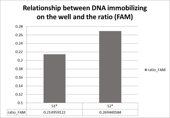
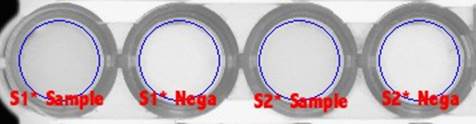
Fig. 12 ::
(TOP) :: Here we illustrate the influence of surface effects on the hybridization rate of S1*-FAM oligonucleotides to one of the two hemispheres of an
asymmetrically functionalized magnetic bead bound to a surface via one of its hemispheres. Specifically, if the bead is bound in a streptavidin coated well
decorated with b-S1* oligonucleotides (in the manner of experiment [1.2]) (LEFT), the FAM signal from S1*-FAM probes is depressed relative to the FAM
signal obtained when beads are coupled to a microarray surface coated with b-S2* strands (RIGHT). Provided the large (
![]() ) diameter of the beads under consider in this study, it is unclear why such a significant effect is observed!
) diameter of the beads under consider in this study, it is unclear why such a significant effect is observed!
(BOTTOM) :: Actual data for microplate scans with equal-size collection and averaging areas indicated with (BLUE) circles. Debris and well edges on the microplate are avoided to the extent possible.
Figure 13: Illustration of “surface effect”-based hindrance of Cy5 probe hybridization to “bichromatic” ferromagnetic beads.
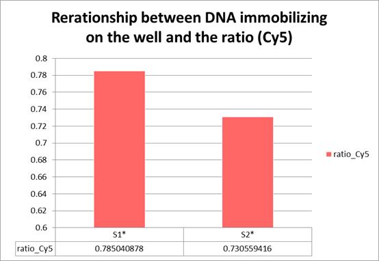
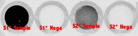
Fig. 13 ::
(TOP) :: Here we illustrate the influence of surface effects on the hybridization rate of S2*-Cy5 oligonucleotides to one of the two hemispheres of an
asymmetrically functionalized magnetic bead bound to a surface via one of its hemispheres. Specifically, if the bead is bound in a streptavidin coated well
decorated with b-S2* oligonucleotides (in the manner of experiment [1.2]) (RIGHT), the Cy5 signal from S2*-Cy5 probes is depressed relative to the Cy5
signal obtained when beads are coupled to a microarray surface coated with b-S1* strands (LEFT). Provided the large (
![]() ) diameter of the beads under consider in this study, it is unclear why such a significant effect is observed!
) diameter of the beads under consider in this study, it is unclear why such a significant effect is observed!
(BOTTOM) :: Actual data for microplate scans with equal-size collection and averaging areas indicated with (BLUE) circles. Debris and well edges on the microplate are avoided to the extent possible.
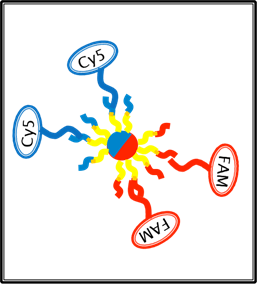
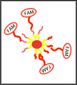
Figure 14: Illustration of bichromatic / asymmetrically functionalized magnetic beads having competency to dock to two microplate wells of distinct “coloration”.
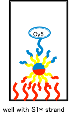

Fig. 14:
Here we show a cartoon illustration the sort of bead docking interactions we expect to be possible for our bichromatic beads. (YELLOW) strands represent
the oligo (b-pT(20)-S3), which, via two sets of bead docking and
![]() UV light exposure steps, can be functionalized on one hemisphere with (CVU-S1) (RED along with its complement) and the other hemisphere with ( CVU-S2) (BLUE along with its complement). This then allows for beads to be:
UV light exposure steps, can be functionalized on one hemisphere with (CVU-S1) (RED along with its complement) and the other hemisphere with ( CVU-S2) (BLUE along with its complement). This then allows for beads to be:
(1; LEFT) Docked to S1* complements in microplate wells, flipping their S2 labeled hemispheres outward, which can be efficiently labeled with S2*-Cy5 probes.
OR
(2; RIGHT) Docked to S2* complements in microplate wells, flipping their S1 labeled hemispheres outward, which can be efficiently labeled with S1*-FAM probes.
1. Detection of completed bi-color DNA beads with fluorescence microscope
We fix another strand (cvU-S2) on the other hemisphere of mag-beads in the same way as step2. Now, A strand is fixed on the north hemisphere of the beads, and B strand is on the south hemisphere. We add S2*-Cy5 DNA to the wells of the microplate, and the hybridization between S2 and S2* DNA will occur. We observe the intensity of the fluorescence if Cy5 is on the surface of the mag-beads.
1. Detection of bi-color beads with the fluorescence microscope
In this experiment, we detected bi-color beads that we made in 4-2. We added S1*-FAM and S2*-Cy5 strand to the beads and hybridized S1 with S2* and S2 with S2*. Because we supposed that S1 and S2 strand were attached to the distinctive hemisphere of the beads, only one hemisphere of the beads would look bright when detected with the fluorescence microscope. Also, when detected by different wavelength range, the other hemisphere would look bright.
Picture 2 Image of Samples
Picture 3 Image of Negative controls
Result
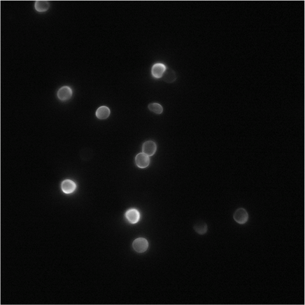
Picture 4 Samples with FAM (x 100)
We can confirm color gradient, the ratio of the brighting part and dark part is 1: 1, from Picture 12.
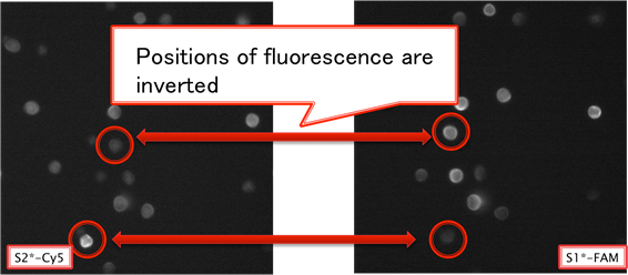
Picture 5 Comparing Sample with FAM and Cy5 (x 100)
From picture 16, we can confirm that the distinctive part of a bead is shining with FAM and Cy5. This is because S1*-FAM and S2*-Cy5 attaches to different part of a bead
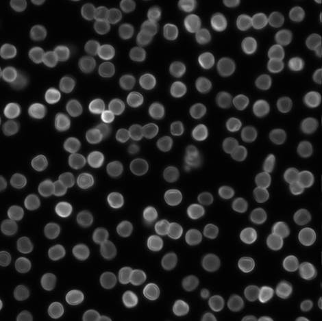
Picture 6 Negative controls with FAM (x 100)
The bead is micrometer scale. So, each bead performs Brownian motion, and Brownian motion involves rotation. If a bead looks bright locally, it doesn’t necessarily means that DNA is attached locally on the surface of beads. In picture 16, some beads look bright locally. In order to exclude this efficient we examined the percentage of beads having gradation of fluorescence about each picture.
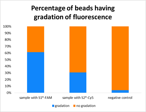
Figure 1
According to Figure 11, the percentage of each Sample is clearly bigger than that of negative control. Therefore, we can say that we could confirm the
beads having gradation of fluorescence due to DNA specific binding.
2. Detection of structures formed by bi-color beads with Bridge strand with the fluorescence microscope
We detected distinctive beads in 4-3. We could confirm place-specific binding of DNA with the surface of beads. So, we detected the linear-structure of bi-color beads. We attached bridge strand like picture 17.

Picture 7 Image of bridge with beads. The green strand is bridge strand. We employed the orthorgal sequence against S1, S2, S3
Result
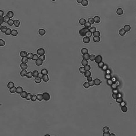
Picture 8 Sample without fluorescence (x 100)
In picture 18, we could confirm the linear structure. Like 3-1, we compare the ratio of Sample with linear structure with that of negative control.
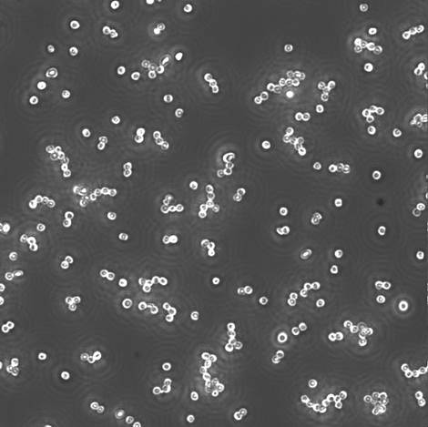
Picture 9 Sample (x 40)
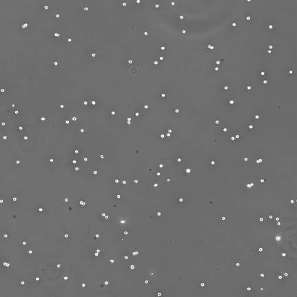
Picture 10 Negative Control (x 20)
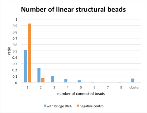
Figure 2
From figure 12, we can know that the ratio of sample with linear structure is bigger than that of the negative control. So, we could make linear structure by using bi-color beads’ specific immobilizing.